Tonight I will be watching the presidential debates. Since I can't stand the commentators on any of the major news networks, I will once again be watching the debates on cspan. If you don't have cable (or your cable plan doesn't include CSPAN), you can watch the video feed online. If you're running Debian, you can also use rtmpdump and mplayer to play the stream on your computer fairly easily:
  rtmpdump -v -r rtmpt://cp82346.live.edgefcs.net:1935/live?ovpfv=2.1.4 \
     --tcUrl rtmp://cp82346.live.edgefcs.net:1935/live?ovpfv=2.1.4 \
     --app live?ovpfv=2.1.4 --flashVer LNX.11,2,202,238 \
     --playpath CSPAN1@14845 \
     --swfVfy http://www.c-span.org/cspanVideoHD.swf \
     --pageUrl http://www.c-span.org/ | \
     mplayer -xy 3 -;
Then you can find a bingo card of your own, and play debate bingo! Or some other horrible drinking game.
In many organisms it is common to use idiograms or cytobands which provide information on approximately where something is located on a chromosome in reference to the chromosome's larger structure, or when exact locations are not required.
Until recently, I didn't know where NCBI
kept their idiogram annotations, which made my
mirror of dbsnp (which I use to annotate my
whole genome analyses) slightly less useful than it could have been.
But, after a bit of searching of NCBI's ftp site, I was able to locate
the file in the new
movie directory:
ideogram_9606_GCF_000001305.13_850_V1.
Then, a quick bit of work with SQL, I have the following schema:
CREATE TABLE idiogram (
       chr TEXT NOT NULL,
       pq  TEXT NOT NULL,
       idiogram TEXT NOT NULL,
       -- I think these are related to recombination rates, but I'm not sure
       rstart INT NOT NULL,
       rstop INT NOT NULL,
       start INT NOT NULL,
       stop INT NOT NULL,
       -- I believe this indicates whether the band is black or white
       posneg TEXT NOT NULL
       );

CREATE UNIQUE INDEX ON idiogram(chr,pq,ideogram);
CREATE UNIQUE INDEX ON idiogram(chr,start);
CREATE UNIQUE INDEX ON idiogram(chr,stop);
and an additional bit of SQL in my SNP annotation perl script:
SELECT CONCAT(chr,pq,idiogram) AS idiogram
  FROM idiogram
  WHERE idiogram.chr = ? AND idiogram.start <= ? AND idiogram.stop < ? LIMIT 1;
and some code:
sub find_idiogram {
    my %param = @_;

    my %info;
    my $rv = $param{sth}->execute($param{chr},$param{pos},$param{pos}) //
    die "Unable to execute statement properly: ".$param{dbh}->errstr;
    my ($idiogram) = map {ref $_ ?@{$_}:()} map {ref $_ ?@{$_}:()} $param{sth}->fetchall_arrayref([0]);
    if ($param{sth}->err) {
    print STDERR $param{sth}->errstr;
    $param{sth}->finish;
    return 'NA';
    }
    $param{sth}->finish;
    return $idiogram // 'NA';
}
and viola:
| id | chr | pos | idiogram | ref | alt | orig_id | gene | [...] |
|---|---|---|---|---|---|---|---|---|
| rs10000010 | 4 | 21618674 | 4p16.3 | T | C | rs10000010 | KCNIP4 | [...] |
idiograms for every SNP.
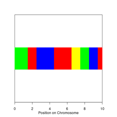
I was asked over the weekend how to plot SNPs which are associated with specific ethnicities; the following code is a really quick stab at the problem using the grid graphics engine in R.
> require(grid)
> snp.position <- 1:10
> snp.integers <- sample.int(5,size=length(snp.position),replace=TRUE)
> ### the position is really the midpoint of the range
> snp.midpoint <- snp.position
> ### start of the SNP; we're assuming it should start at 0.
> snp.start <- c(0,snp.position[-1]-diff(snp.position)/2)
> ### stop of the snp; we're assuming it should stop at the last snp position
> snp.stop <- c(snp.position[-length(snp.position)]+diff(snp.position)/2,
>   snp.position[length(snp.position)])
> snp.width <- snp.stop - snp.start
>
> ### these are the colors
> possible.colors <- c("red","blue","yellow","green","purple")
> snp.colors <- possible.colors[snp.integers]
>
> ### this sets up the viewport that we'll plot into
> pushViewport(viewport(height=unit(1,"npc")-unit(7,"lines"),
> width=unit(1,"npc")-unit(7,"lines")
>   ))
> pushViewport(dataViewport(xscale=range(c(0,snp.stop)),yscale=c(0,1)))
>
> ### this draws a rectangle around the graph
> grid.rect()
> ### this sets up the x axis
> grid.xaxis()
> ### this labels the X axis
> grid.text("Position on Chromosome",y=unit(-2.5,"lines"))
>
> ### this draws all of the boxes corresponding to each SNP in the
> ### appropriate color
> grid.rect(x=unit(snp.start,"native"),
>         width=unit(snp.width,"native"),
>         y=unit(0.5,"native"),
>         height=unit(0.25,"native"),just=c("left","center"),
>         gp=gpar(col=snp.colors,fill=snp.colors))
>
> ### this pops the viewport
> popViewport(2)
Christian's most recent blog post
got me wondering if the decline in the bug reporting rate in Debian
was something new, or something which often happened during releases.
So, lets try to figure that out. In the BTS, when a bug report is
filed, the report is written to a file called bugnum.report, and
then not touched from then on. Let's look at the modification date on
that file to see when each bug was filed; and since we're going to
plot this, lets only look at bugs ending in 00:
stat -c '%n %Y' /srv/bugs.debian.org/spool/{archive,db-h}/00/*.report > ~/reporting_rate.txt
Now, lets get the data into R and plot it. [For clarity, I'm not showing the R code, but it's available in the source code for this post.]
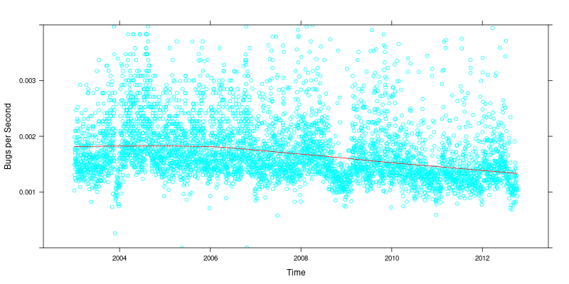
From the plot (Bugs reported per second over time with a red loess fit line), it looks like we do see a decline during certain periods. However, there's an even more alarming trend of a decrease in bug reporting in Debian which has been happening since 2006. (Note that I've truncated the y scale significantly; there are periods in Debian where the bug rate is astronomically high, usually corresponding to mass bug filings; I've also limited the plot to data from 2003 on, as I have to clean up that data significantly before I can plot it like this.)
Not sure exactly what that means, but it is troubling.